How To Count Highlighted Cells In Excel

6 Ways to Count Colored Cells in Microsoft Excel [Illustrated Guide]

You have probably used color coding in your Excel data or seen information technology in a workbook you had to utilise.

Information technology'south a popular manner to visualize your data!

While colored cells are a great mode to highlight data to quickly grab someone's attending, they are not a slap-up mode to shop data.

Unfortunately, a lot of users will colour a cell to indicate some value instead of creating another data point with the value.

For example, they might color a cell green to signal an item is canonical instead of creating another information betoken with the text Approved.

This causes a lot of problems when yous actually demand to find out how many items were approved. Excel doesn't offer a congenital-in way to count colored cells.

In this post, I'll show you 6 ways to find and count any colored cells in your data.

Use the Find and Select Control to Count Colored Cells

Excel has a cracking characteristic that allows yous to find cells based on the format. This includes any colored cells likewise!

You tin can find all the cells of a certain color, then count them.

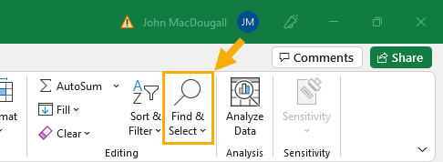
Go to the Home tab ➜ click on the Find & Select control ➜ and so choose Notice from the options.

There is besides a corking keyboard shortcut for this. Press Ctrl + F to open up the Detect and Replace menu.

Click on the minor down arrow in the Format button and select Choose Format From Cell.

Clicking on the main part of the Format push will open the Find Format menu where you can select whatsoever combination of formatting to search for.

This is perfect if you know exactly what color you are searching for, but more than ofttimes yous volition be best served by setting the format by example. Formatting could exist subtilty dissimilar and this might cause yous to miss finding the right data!

When you lot click on the small arrow inside the Format push button, information technology volition reveal more options including the ability to prepare the format by selecting a prison cell.

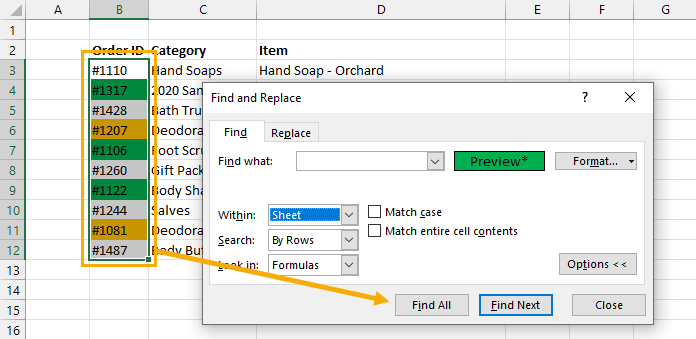
Once you have the format selected then click on the Find All push.

The lower office of the Detect and Replace dialog box will show all the cells that were found matching the formatting and in the lower left you will find the count.

Press Ctrl + A to select all the cells then press the Close button and you can then change the color of all these cells or modify whatsoever other formatting.

If you but desire to return cells in a given cavalcade, or range, this is possible. Select the range in the canvass before pressing the Find All button to limit the search to the option.

Pros

• Easy to use.
• Y'all can apply this to search for other types of formatting and non just fill color.
• You can utilise this to search a selected range, the unabridged sheet or the entire workbook.

Cons

• This solution is not dynamic and will demand to be repeated each fourth dimension you desire to get the count.

Use Filters and the Subtotal Office to Count Colored Cells

This method will rely on the fact that you can filter based on cell color.

First step, y'all will need to add filters to your data.

Select you information and go to the Information tab and then choose the Filter command.

This will add a sort and filter icon to each cavalcade heading of your data and these will allow you lot to filter your information many different means.

There is likewise a handy keyboard shortcut for adding or removing filters from your data. Select your data and press Ctrl + Shift + L on your keyboard.

Another selection for adding filters is to turn your data into an Excel Table. I wrote a mail service all about Excel tables and the great features they come with.

Y'all can catechumen your data into a table with either of these two methods.

• Select a cell within your data ➜ go to the Insert tab ➜ click on the Tabular array command.
• Select a cell inside your data ➜ press Ctrl + T on your keyboard.

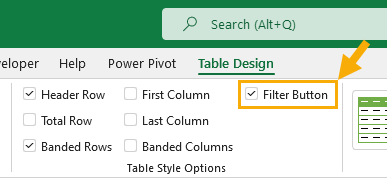
Y'all table should come with filters by default. If not, get to the Table tab and check the Filter Button option in the Tabular array Style Options section.

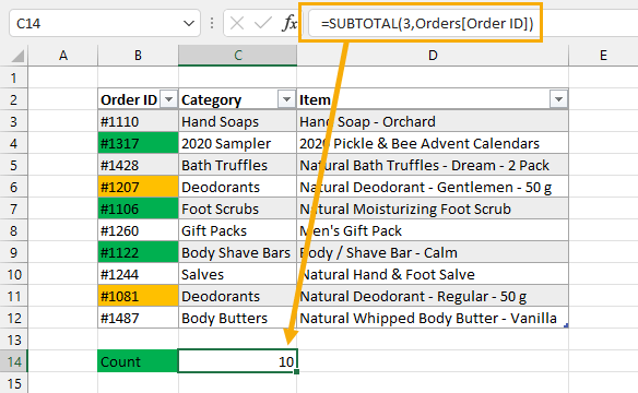
          = SUBTOTAL ( 3, Orders[Order ID] )        

At present you lot can add the in a higher place SUBTOTAL formula to count the non empty cells where Order ID is the column which contains the colored cells you lot would like to count.

The get-go statement of the SUBTOTAL function tells it to return a count while the second argument tells information technology what to count.

The special trick here is that the SUBTOTAL function volition only count visible cells, so it will update the count based on what data information technology is filtered on.

This ways y'all can filter on the colored cells and you volition get a count of those colored cells!

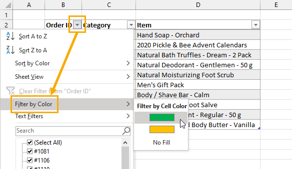
At present you can filter your data past color.

1. Click on the sort and filter toggle for the column which contains the colored cells.
2. Select Filter by Colour from the menu options.
3. Choose the color you want to filter on.

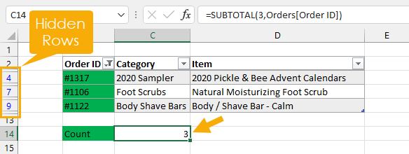
Now the SUBTOTAL upshot volition update and you can quickly find the count of your colored cells.

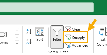
If y'all arrange colors, add or delete data in the table. You will need to reapply the filters equally they don't update dynamically.

Go to the Data tab and click on the Reapply button in the Sort & Filter section.

Pros

• Piece of cake to use.

Cons

• Requires manually filtering data.
• The filters don't update and you will need to reapply them when yous change your data.
• Since the count is based on the filtering, the consequence can be different for each user when collaborating on the workbook.

Use the Become.Prison cell Macro4 Function to Count Colored Cells

Excel does have a role to become the fill up color of a jail cell, simply it is a legacy Macro 4 function.

These predate VBA and were Excel's formula based scripting language.

While they are considered deprecated, it is still possible to use them inside the name manager.

In that location is a Go.CELLS Macro4 role that will return a color code based on the fill color of the cell.

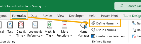
You lot tin create a relative named range that uses this by going to the Formulas tab and clicking on Define Proper name.

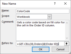
This will open upwardly the New Name menu and you tin define the reference.

Give your defined proper name a Name similar ColorCode. This is how you volition refer to it in the workbook.

          = GET.Cell ( 38, Orders[@[Order ID]] )        

Add the to a higher place formula into the Refers to section. For this formula y'all information will need to be in a table named Orders with a column chosen Guild ID, only you lot can change these to fit your data.

This formula will always refer to the Order ID jail cell in the current row to which it's referenced.

          = GET.CELL ( 38, $B3 )        

If your data is not inside a table, so you could use the above formula instead, where B is the column containing the fill colour you want to count. This uses a fixed cavalcade and relative row reference to always refer to column B of the current row.

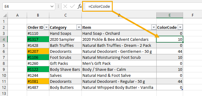
          = ColorCode        

With the define proper noun, you can now create another column using the above formula in your data to calculate the color code for each row.

The result will exist an integer value based on the make full color of the cell in the Guild ID column.

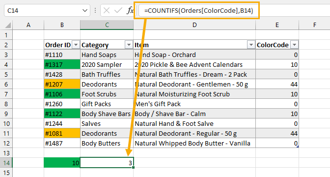
          = COUNTIFS ( Orders[ColorCode], B14 )        

At present you can count the number or colored cells using the in a higher place COUNTIFS formula.

This formula will count cells in the ColorCode column if they accept a matching code. In this example, it counts all the 10 values which correspond to the dark-green color.

Pros

• You tin can calculate the make full color for each row of information and it will update dynamically every bit y'all change the data or make full color of the data.

Cons

• This method uses the Macro4 legacy functions and they may not keep to be supported my Microsoft.
• Harder to implement.
• You will need to salve your workbook in the xlsm macro enabled format.
• You can't move your referenced cavalcade if you're using the cavalcade annotation inside the named range.
• You can't alter your column name if you're using the table notation within the named range.
• You need to create an additional cavalcade and utilise a COUNTIFS function to become the count.

Employ a LAMBDA Function to Count Colored Cells

This will use the same Become.CELL Macro4 function as the previous method, but you tin can create a custom LAMBDA function to employ it inside the workbook.

The LAMBDA function is a special function that allows you lot to build custom functions via the proper noun manager.

This is a new function, so it's not more often than not bachelor and you need to be on Microsoft 365 function insiders program at the fourth dimension of writing this post.

Go to the Formulas tab and click on Define Proper name to open up the New Proper name carte.

          = LAMBDA ( jail cell, Become.CELL ( 38, cell ) )        

Give the ascertain name a name like GETCOLORCODE and add the higher up formula into the Refers to section.

This will create a new GETCOLORCODE office that you tin utilise inside the workbook. It volition take ane statement called cell and return the cell's fill color lawmaking.

          = GETCOLORCODE ( [@[Society ID]] )        

Now all yous have to do is create a column to calculate the colour code for each row using the to a higher place formula.

          = COUNTIFS ( Orders[ColorCode], B14 )        

Once again, you tin count the number or colored cells using the the above COUNTIFS formula.

Pros

• You tin can build a role that calculates the color code for a given cell.
• Allows you to straight reference a prison cell to get the color lawmaking.

Cons

• This method uses the LAMBDA role in Excel for M365 and is currently non mostly available.
• Harder to implement.
• This method uses the Macro4 legacy functions which may non be supported in the future.
• You will need to relieve your workbook in the xlsm macro enabled format.
• Requires creating an additional cavalcade and using a COUNTIFS role to go the count.

Use VBA to Count Colored Cells

          Office COLORCOUNT(CountRange Every bit Range, FillCell As Range) Dim FillColor Equally Integer Dim Count As Integer FillColor = FillCell.Interior.ColorIndex For Each c In CountRange     If c.Interior.ColorIndex = FillColor Then         Count = Count + ane     End If Next c COLORCOUNT = Count End Function        

Pros

• You tin create a function that counts the colored cells in a range.
• The results will update as yous edit your data or modify the fill color.
• User friendly option to use once it is fix.

Cons

• Uses VBA which requires the file is saved in the xlsm format.
• Less user friendly to prepare up.

Utilise Office Scripts to Count Colored Cells

Role Scripts are the brand new method for automating tasks in Excel.

But it's only available for Excel online and only with an enterprise program. If you have an enterprise plan, and then you're adept to go with this method!

Offset, y'all will need to set up two named cells which the code volition refer to.

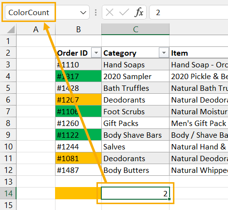
Select any jail cell and type a proper noun like ColorCount into the name box and press Enter. This will create a named range which can be referred to in the code.

This ways we can motility the cell and the code volition refer to its new location.

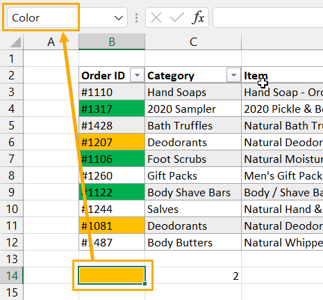
You will too need to create a Colour named range for the input of the color to count.

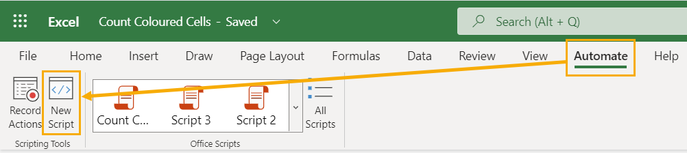
Now you can create a new function script. Get to the Automate tab in Excel online and click on the New Script control.

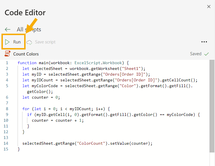
          function master(workbook: ExcelScript.Workbook) { 	let selectedSheet = workbook.getWorksheet("Sheet1"); 	let myID = selectedSheet.getRange("Orders[Order ID]"); 	let myIDCount = selectedSheet.getRange("Orders[Club ID]").getCellCount(); 	let myColorCode = selectedSheet.getRange("Color").getFormat().getFill().getColor(); 	let counter = 0;  	for (let i = 0; i < myIDCount; i++) { 		if (myID.getCell(i, 0).getFormat().getFill().getColor() == myColorCode ) { 			counter = counter + 1; 		}  	}  	selectedSheet.getRange("ColorCount").setValue(counter); }        

This will open up the Lawmaking Editor and you can paste in the above code and salve the script.

Press the Run push button and the code volition execute and then populate the ColorCount named range with the count of the colored cells institute in the Order ID column.

Pros

• This is the newest method and will exist supported going forward.
• The script tin can be run from Power Automate for a no click solution.

Cons

• This method is difficult to fix.
• This requires an enterprise license and yous need to use Excel online.

Conclusions

Hopefully Microsoft volition one day create a standard Excel function that can render properties from a cell such as its fill colour.

Until that happens, at least you have a few options available that allow you to observe the count of colored cells without manually counting them.

Do you have a preferred method not listed here? Let me know in the comments!

About the Author

John is a Microsoft MVP and freelance consultant and trainer specializing in Excel, Power BI, Power Automate, Power Apps and SharePoint. You can observe other interesting articles from John on his blog or YouTube channel.

Source: https://www.howtoexcel.org/count-colored-cells/

Posted by: buzzellyoublearded.blogspot.com

Share this post